When two distributions are
better than one: Mixture models and word frequency distributions.
Fiona J. Tweedie
Department of Statistics
Mathematics Building
University Gardens
GLASGOW, Scotland G12 8QW
fiona@stats.gla.ac.uk
Harald Baayen
University of Nijmegan
Max Planck Institute for Psycholinguistics
Wundtlaan 1
PB 310, 6500 AH NIJMEGEN
The Netherlands
baayen@mpi.nl
Summary
Models for word frequency distributions are relevant for a wide range of
domains of inquiry, including authorship studies, statistical language
engineering, theoretical linguistics, and linguistic synergetics. For
inferences based on such models to be useful, they should provide accurate
descriptions of the data to which they are fitted. This paper shows that
improved fits may sometimes be obtained by analysing word frequency
distributions as mixtures of two or more distinct component distributions, with
the gain in accuracy outweighing the increased number of model parameters.
Introduction
Currently, there are three models for word frequency distributions
available that take the dynamics of the development of spectral
characteristics as a function of sample size into account: the
lognormal model, the extended generalized Zipf's model, and the
generalized inverse Gauss-Poisson model (GIGP), see Chitashvili and
Baayen (1993), for a review of these LNRE models. Although many
empirical word frequency distributions are well-described by one or
more of these models, there are also word frequency distributions for
which no adequate fit is available. Baayen and Tweedie (1998) discuss
informally a data set concerning the frequencies of use of Dutch words
with the suffix -heid (cf. -ness in English) which
illustrates this point.
The word frequency distribution of -heid is problematic because
the medium frequency ranges of the spectrum are more densely populated
than expected by the LNRE models. This suggests that we might be
dealing with a mixture of two, or more, distributions, rather than
with a single homogeneous distribution. The question we have set
ourselves is: Is it possible to find two component LNRE models that
jointly provide an improved fit to the observed frequency spectrum of
-HEID?
Mixture Models
Mixture models describe distributions where the data can be drawn from
one or more sources. Our starting point is a word frequency
distribution spectrum without any indication of how it is to be
decomposed into its two components. In general, when we model a word
frequency spectrum we are interested in finding expected values of the
elements V(m,N), the number of words occurring m times in a text of
length N. The parameters of LNRE models are then chosen to make the
expected value of the spectrum elements, E[V(m,N)] as close to the
observed V(m,N) as possible. When a single distribution is not enough
to deal with the observed data, we can consider the use of a mixture
distribution, where the expected values are made up as follows:
- E[V(m,N)] = E_1[V(m,pN)] + E_2[V(m,(1-p)N)],
where p is the proportion of the data coming from the first
distribution, usually called the mixing parameter, and (1-p) the
proportion which comes from a second distribution. E_1 and E_2
indicate the expected values under the different distributions.
It can be shown for each of the LNRE models that
- E[V(m,pN)|Z,...] = p E[V(m,N)|Z/p,...]
with Z the LNRE parameter of the distribution. This general relation,
which expresses a form of self-similarity in word frequency
distributions, allows us to show that limiting properties of the
mixture, such as its estimated population number of types, is the sum
of its mixture components. Similarly, expressions of variances and
covariances of the spectrum elements can be derived, so that the
mixture model itself is again a complete LNRE model.
-HEID as a Mixture Distribution
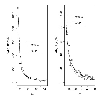
Figure 1 plots the number of types V(m,N) with frequency m in a sample
of size N as a function of m, for m = 2, ..., 15 in the left panel,
and for m=15, ..., 100 in the right panel, using dots (N=167353). The
dashed line represents the GIGP fit to the data (\hat{Z} = 41.5554,
\hat{b} = 0.00765648, \hat{\gamma} = -0.446889), which overestimates
for low m and underestimates for larger m. Other LNRE models provide
even worse fits to the data. The solid line represents the mixture
model for a Lognormal component (\hat{Z} = 200, \hat{\sigma} = 2.05)
and a GIGP component (\hat{b} = 0.000000002093, \hat{Z} = 82.9848,
\hat{\gamma} = -0.565). The mixing parameter p equals 0.96. The MSE
(mean squared error) for the GIGP fit is 3390.6, and X^{2}(13) =
1734.7, p < .1*10^-18. For the mixture model, the MSE is reduced to
97.1, and with X^{2}(10) = 19.58, p=0.0334 we have no reason to reject
the model. We have obtained similar improvements in goodness-of-fit
for other word frequency distributions that thusfar resisted adequate
modeling. At the conference, we will present further examples of the
advantages of using mixture models where `pure' models fail, and we
will demonstrate the software that we have been developing to fit
mixture LNRE models to empirical data.

References
- Baayen, R. H. and Tweedie, F.J.: 1998, "Mixture models and word frequency
distributions." Abstracts of the ALLC/ACH Conference, Debrecen, July 1998.
- Chitashvili, R. J. and Baayen, R. H.: 1993, "Word Frequency Distributions,"
In: G. Altmann and L. Hrebicek, L. (Eds.), Quantitative Text Analysis,
Wissenschaftlicher Verlag Trier, Trier, pp. 54-135.

